
When does frequency decomposition help physics-informed neural networks?
Shubham Rai, a research intern at Bibha, built a dual-branch, spectrally gated PINN purely so that each part could be switched off. The ablation shows frequency decomposition paying off on multi-scale wave problems and adding nothing, or worse, on smooth single-scale ones.
What question does the paper ask?
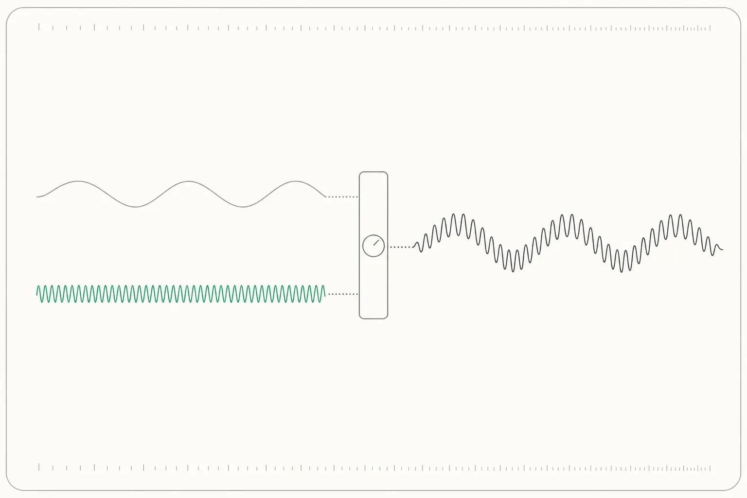
The paper asks when frequency decomposition actually improves a physics-informed neural network, rather than assuming it always does. Shubham Rai, a research intern at Bibha supported by the engineering team, answers it with a controlled ablation across five one-dimensional PDE benchmarks of rising spectral complexity.
Physics-informed neural networks, or PINNs, fold a governing equation and its boundary and initial conditions into the training loss, so a network has to satisfy the physics rather than fit observed data alone. They are now a default tool in scientific machine learning, but they inherit a well-known weakness of gradient-trained networks: spectral bias. Low-frequency parts of a solution are learned quickly, high-frequency parts slowly or not at all.
A family of fixes exists, from Fourier feature embeddings and sinusoidal activations to domain decomposition and gating. Most of that work argues that richer spectral representations help in general. The paper takes the opposite stance: physical systems differ widely in spectral character, so the benefit should depend on the problem. Few studies had compared frequency-aware architectures against matched ablations across PDEs of different complexity, and that gap is what the study sets out to fill.
The DBSG-PINN architecture, built to be taken apart
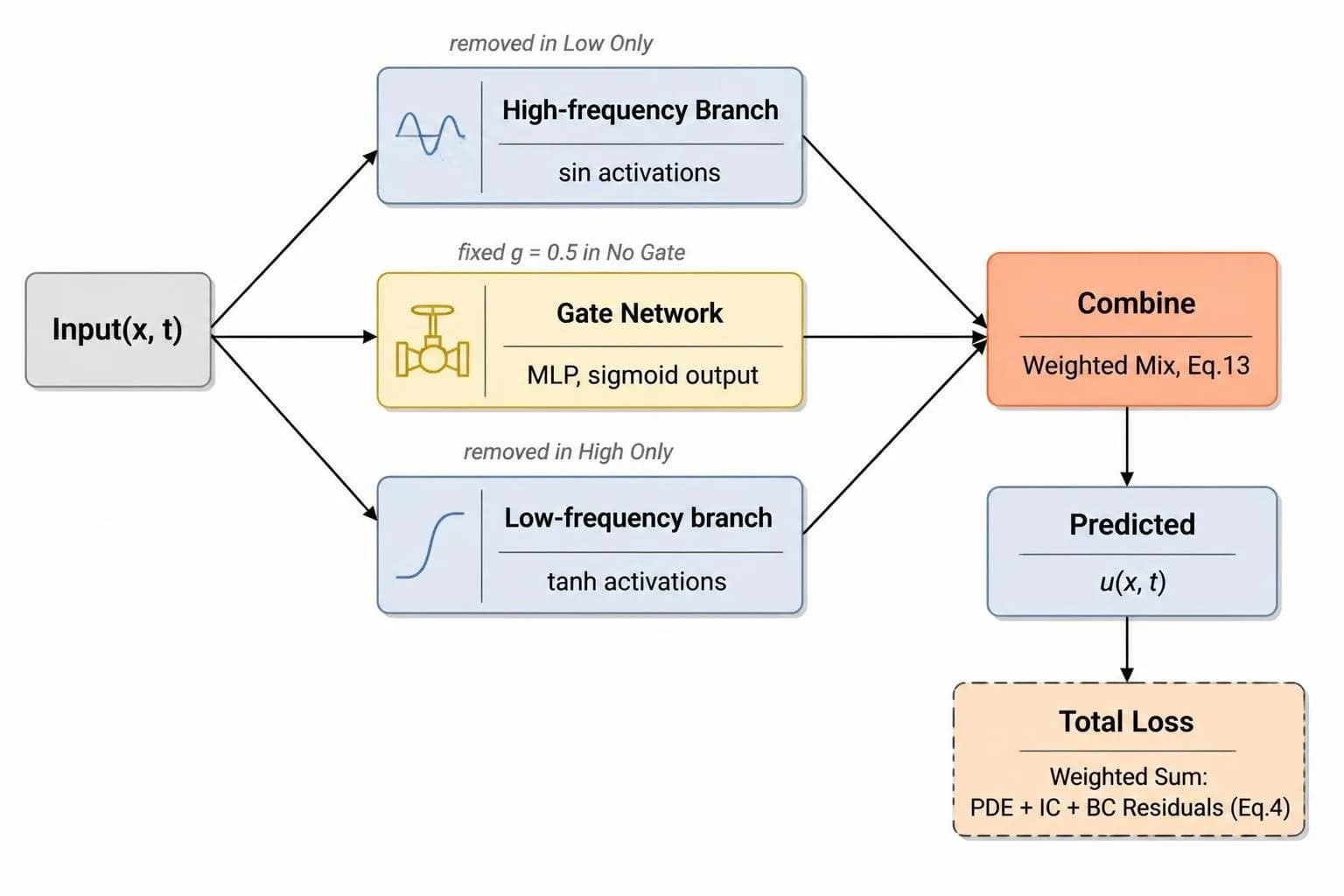
DBSG-PINN, the Dual-Branch Spectral-Gated PINN, splits the approximation into two subnetworks and a learned gate, and every component can be removed without touching the optimiser. That design choice is the point: it turns the architecture into an instrument for ablation rather than a product.
The low-frequency branch uses hyperbolic tangent activations, the classical smooth nonlinearity, to capture gentle solution components. The high-frequency branch uses sinusoidal activations in the style of SIREN networks to represent oscillatory, multi-scale behaviour. Both branches receive the same space and time coordinates and train jointly, end to end, with nothing pretrained or frozen.
A small gate network produces a sigmoid value between 0 and 1 at every point in space and time. The final prediction is a convex combination: the gate weight times the high-frequency branch plus one minus that weight times the low-frequency branch. Because exactly two branches are mixed, a scalar sigmoid replaces the softmax used in mixture-of-experts models.
The author is careful about language. The branch names describe an intended inductive bias from the activation function, not a formal spectral split. Nothing stops either branch from representing any function its depth allows; the gate decides how much each contributes where.
How were the ablation variants constructed?
Each variant is the same computational graph with one component structurally removed or fixed, trained from a fresh initialisation while the optimiser, iteration count, collocation points and loss weights stay exactly as in the full model for that benchmark. Only the active architectural pieces change.
The four variants probe two questions. Full against NoGate asks whether a learned gate beats a fixed average, since NoGate pins the gate at 0.5. LowOnly and HighOnly against Full ask whether a single frequency regime is enough, by dropping the high-frequency branch or the low-frequency branch respectively.
The paper states a limitation up front rather than burying it. The two branches are only roughly capacity-matched: on most benchmarks the high-frequency branch is wider, for example 64 against 32 units on Multimodal Wave and 128 against 64 on 1D Wave, and depth differs by a layer or two elsewhere. So LowOnly against HighOnly is not a clean test of tanh against sine on its own. Even equal parameter counts would not guarantee equal expressivity between the two activation families.
Training follows common PINN practice: an Adam phase for rapid descent, then L-BFGS to refine near the minimum. Loss weights are fixed per benchmark so all variants share one loss landscape.
- Full. Both branches active, mixed by the learned gate at every point in space and time.
- NoGate. Both branches active, but the gate is fixed at 0.5, giving a plain average of the two outputs.
- LowOnly. The high-frequency branch and the gate are removed; the prediction is the tanh branch alone.
- HighOnly. The low-frequency branch and the gate are removed; the prediction is the sine branch alone.
Five benchmarks and six metrics
The benchmarks were chosen to span spectral complexity: Burgers, Reaction-Diffusion, Allen-Cahn, the standard 1D Wave equation and a Multimodal Wave equation whose solution superposes three spatial modes. Each was evaluated on a uniform 100 by 100 grid in space and time.
Multimodal Wave is the spectrally richest case. Its initial condition combines modes 1, 3 and 5 with amplitudes 1.0, 0.7 and 0.4, and the closed-form solution keeps all three modes oscillating in time. At the other end sit Reaction-Diffusion, a single sine profile that grows or decays, and 1D Wave, a single mode at wavenumber 4. Burgers is smoothed by viscosity to something close to single-scale, and Allen-Cahn is smooth apart from sharp, localised transition layers.
Accuracy is reported as relative L2 error and maximum pointwise error, following the convention introduced with the original PINN paper and adopted by the DeepXDE library. A mean PDE residual, computed after training with finite differences on the evaluation grid, acts as a consistency check rather than a measure of the quantity the optimiser minimised.
Three spectral diagnostics adapt the Fourier-domain view of spectral bias to a trained solution. The amplitude spectrum of the prediction is compared with that of the reference over wavenumbers up to 20, excluding the mean level. Modes 2 to 5 form a low-frequency band and modes 6 to 20 a high-frequency band, each summarised by a recovery score that reaches 1 when the spectra match. The author flags that on single-mode benchmarks the high-frequency band holds almost no reference energy, so its recovery score behaves as a noise-floor diagnostic rather than an accuracy measure.
What did frequency decomposition change on each benchmark?
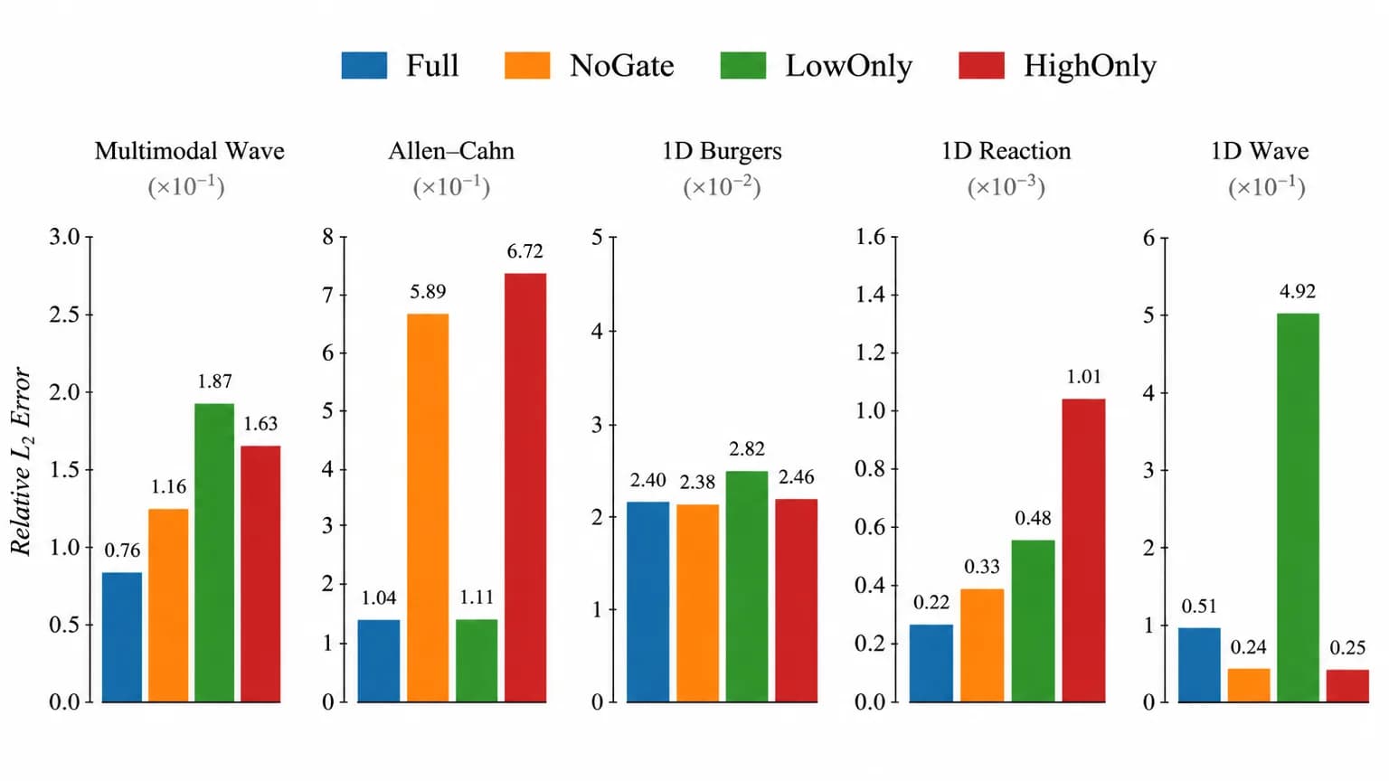
Decomposition helped most on the genuinely multi-scale target and least on the simplest ones. On Multimodal Wave the full model led every ablation on nearly every metric, with relative L2 error of 0.0762 against 0.1161 for NoGate, 0.1869 for LowOnly and 0.1632 for HighOnly, the source of the up to 59.2% improvement quoted in the abstract.
Allen-Cahn was closer. Full stayed ahead of LowOnly, 0.1038 against 0.1108 in relative L2 error, while NoGate and HighOnly fell far behind. The interpretation offered is that the gate's job here was to suppress a sinusoidal branch that did not fit a mostly smooth solution, rather than to blend two useful branches, and that a different seed could plausibly flip the narrow Full-to-LowOnly ordering.
Burgers was a wash. Full and NoGate finished within a few thousandths of each other on relative L2 error, 0.0240 against 0.0238, with each variant ahead on about half the columns and by under 5% either way. Viscosity leaves little spectral structure for a gate to route between.
Reaction-Diffusion is the awkward case. Its solution is a single spatial mode, yet the full model still led on every accuracy metric. The author declines to force this into the spectral-complexity story and records it as an open question.
1D Wave went the other way, and not by a little. NoGate beat the full model on every tracked metric, by around 53% on relative L2 error and 68% on spectral error. With a single wavenumber there was nothing for the gate to route between, and learning one actively hurt compared with a fixed average. The paper offers no confident explanation and names a multi-seed follow-up as the priority.
| Benchmark | Full (gated) | NoGate | LowOnly | HighOnly |
|---|---|---|---|---|
| Multimodal Wave | 0.0762 | 0.1161 | 0.1869 | 0.1632 |
| Allen-Cahn | 0.1038 | 0.5892 | 0.1108 | 0.6717 |
| Burgers | 0.02398 | 0.02383 | 0.02816 | 0.02455 |
| Reaction-Diffusion | 0.000224 | 0.000325 | 0.000477 | 0.00101 |
| 1D Wave | 0.05134 | 0.02397 | 0.49170 | 0.02514 |
What does the gate's behaviour suggest?
Taken across benchmarks, the gate's benefit scaled with spectral richness: largest on Multimodal Wave, smaller but positive on Allen-Cahn, roughly neutral on Burgers and negative on 1D Wave. That ordering is consistent with a gate that exploits frequency structure rather than adding noise.
The author is explicit that this is inferred from aggregate comparisons, not from inspecting the gate's spatial activations. A direct visualisation of the gate value against local spectral content is listed as a prerequisite before calling the pattern a property of the architecture. Reaction-Diffusion, where the gate helped despite a single-mode target, stands as the counterexample that keeps the claim preliminary.
Why the paper calls itself preliminary
Three limitations bound the findings, and the paper names them rather than leaving readers to find them. Every result comes from a single training seed, so there is no variance estimate; the narrow Allen-Cahn gap and the large 1D Wave gap are both exposed to that uncertainty.
Branch capacity is only roughly matched, and even matched sizes would not equate functional capacity between tanh and sine networks. All five benchmarks are one-dimensional, so nothing is claimed about higher dimensions or stronger nonlinearity.
The acknowledgements are equally direct: the two overview figures were produced with an AI diagramming tool and the manuscript text was refined with an AI assistant, with the author reviewing every output and taking responsibility for the research itself.
What comes next, and why it matters for applied AI
The stated next step is repeating the ablation across multiple seeds to see whether the orderings hold. Beyond that, the paper proposes extending to two-dimensional and time-dependent multi-scale PDEs, building a lightweight diagnostic from the spectral content of initial and boundary data to predict whether decomposition will help, and testing the gate as an interpretability signal beyond this architecture.
For teams building models on Bibha, the method matters as much as the result. Treating an architecture as an instrument, holding the optimiser fixed, removing one component at a time and reporting the cases where the richer design lost are the same habits our platform encourages through its evaluation and release-decision tooling. Comparing a candidate with a baseline on representative cases, and keeping the evidence behind a decision, applies to a PINN exactly as it applies to a business workflow model.
Questions and answers
What is spectral bias in physics-informed neural networks?
Spectral bias is the tendency of gradient-trained neural networks to learn the low-frequency components of a target function well before its high-frequency components. For PINNs it shows up as trouble with sharp gradients, oscillations and solutions that mix several spatial or temporal scales. Fourier features, sinusoidal activations, adaptive losses and domain decomposition are the usual remedies, and this paper asks when such remedies actually pay off.
What is DBSG-PINN?
DBSG-PINN is the Dual-Branch Spectral-Gated physics-informed neural network introduced in the paper. A tanh branch models smooth components, a sine-activated branch models oscillatory components, and a small gate network blends them point by point with a sigmoid weight. Each component can be removed without changing the optimiser, which is what makes the architecture suitable for a controlled ablation study.
Does frequency decomposition always improve PINN accuracy?
Not in this study. On the spectrally rich Multimodal Wave benchmark the full gated model cut relative L2 error by up to 59.2% against the ablations. On Burgers a learned gate and a fixed average were indistinguishable, and on the single-mode 1D Wave benchmark the fixed average won by around 53%. The reported pattern is that benefit tracks spectral complexity, with one seed per result and Reaction-Diffusion as an open exception.
How should the results be used in practice?
As a testable hypothesis rather than a rule. Before adopting a frequency-decomposed PINN, inspect the spectral content of the problem and run a matched ablation on representative cases, exactly as the paper does. If the solution is smooth and single-scale, a simpler model may match or beat the gated design, and a multi-seed comparison is needed before any ordering is trusted.
References
- Rai, S. (2026). When Does Frequency Decomposition Benefit Physics-Informed Neural Networks? A Preliminary Ablation Study. arXiv:2608.24940. https://arxiv.org/abs/2608.24940 (external site)
- Raissi, M., Perdikaris, P. and Karniadakis, G. E. (2019). Physics-informed neural networks: A deep learning framework for solving forward and inverse problems involving nonlinear partial differential equations. Journal of Computational Physics, 378, 686 to 707. https://doi.org/10.1016/j.jcp.2018.10.045 (external site)
- Rahaman, N. et al. (2019). On the spectral bias of neural networks. Proceedings of the 36th International Conference on Machine Learning, PMLR 97. https://proceedings.mlr.press/v97/rahaman19a.html (external site)
- Tancik, M. et al. (2020). Fourier features let networks learn high frequency functions in low dimensional domains. Advances in Neural Information Processing Systems 33. https://arxiv.org/abs/2006.10739 (external site)
- Sitzmann, V. et al. (2020). Implicit neural representations with periodic activation functions. Advances in Neural Information Processing Systems 33. https://arxiv.org/abs/2006.09661 (external site)
- Lu, L., Meng, X., Mao, Z. and Karniadakis, G. E. (2021). DeepXDE: A deep learning library for solving differential equations. SIAM Review, 63(1), 208 to 228. https://doi.org/10.1137/19M1274067 (external site)